
Introduction
Last time, we analyzed the first of several components of IMU preintegration in ORB-SLAM3, the IMU sensor measurement integration part, by comparing the paper and the code. The measurement integration part (1) computes the relative state (rotation, translation, velocity) values between two keyframes, (2) obtains the covariance matrix through noise propagation, and (3) computes the Jacobian matrix for bias update. The values computed here are later used to perform bundle adjustment using keyframes, or to perform nonlinear optimization such as pose estimation for a single camera frame.
In this tutorial, we will analyze how the residual function of IMU factors and the definition of Jacobian matrix are implemented in the ORB-SLAM3 code to perform nonlinear optimization.
Prerequisites
Factor Graphs and MAP Esimation
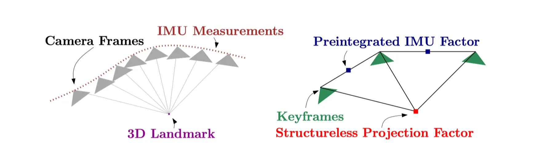
A factor graph is a structure used to represent the relationships between variables in a stochastic model and to find solutions that satisfy all constraints (factors). It is used here to address the Visual-Inertial Odometry (VIO) problem and consists of the following main components
1.
Graph node
a.
Variable node: represents the state of the system (state, )
b.
Factor nodes: represent probabilistic factors that represent relationships between measurements (measurement, ) and states.
2.
Graph edges
a.
Connects variables and factors, and represents constraints on which variables affect which factors.
The VIO problem defined in the IMU preintegration paper is represented as follows in Equation (25).
where the state value the state for the keyframe we are interested in obtaining (rotation , translation , velocity , bias ) values, and the measurements contain observations from the camera sensors (2D keypoint position information about 3D landmarks) and measurements from the IMU sensors (acceleration and angular velocity ). For more details on the notation, please refer to the section IV. Maximum a Posteriori Visual-Inertial State Estimation in the paper.
We want to perform Maximum-a-Priori (MAP) estimation to find the state value that causes the probabilistic model in Equation (25) to have a maximum value. To do this, we take the negative logarithm of Equation (25) and express it in sum form as follows
where are the residuals for the prior factor, the residual for the IMU sensor, and the residual for the Camera sensor, respectively. Here, residual is the difference between the measurement from the sensor and the prediction of the state. Finding the parameter that minimizes the equation (26) composed of these residual functions becomes the solution of the probabilistic model equation (25), and finding this solution is called state estimation of the system.
Nonlinear optimization & Open-source libraries
The process of finding the solution usually uses nonlinear optimization methods, and there are many open-source libraries available for general developers and engineers to easily use, including
•
Google, ceres-solver(http://ceres-solver.org/)
•
Georgia Tech, GTSAM(https://gtsam.org/)
•
University of Freiburg, g2o(https://github.com/RainerKuemmerle/g2o)
•
Skydio, Symforce(https://symforce.org/)
In the ORB-SLAM3 code referenced in this article, the g2o library is used to perform nonlinear optimization, so the code description below will be based on g2o. The tools required in the general nonlinear optimization process (e.g., optimization loop, nonlinear solver, etc.) are all implemented in the library, but the system model of the problem we want to solve must be implemented by ourselves. Therefore, it is necessary to implement the system model for the IMU preintegration problem in code, and what we need is a definition of the residual function and a definition of the Jacobian matrix. In the code analysis section below, we will compare the code in ORB-SLAM3 with the formulas in the IMU integration paper to see how they are implemented.

If you are unfamiliar with nonlinear optimization theory, you may want to take a look at section 03. Non-linear optimization theorem in my book Understanding and Implementing SLAM with NVIDIA Jetson Nano:-)
Code Analysis
Definition of Residual Function
As we briefly explained earlier, the residual function is the difference between the measurement from the sensor and the prediction of the state. The state of the system where this residual value is minimized is calculated using nonlinear optimization. The residual function for IMU preintegration defined in the paper is described in Equation (45). In order, they represent the residuals for the rotation parameter, for the velocity parameter, and for the translation parameter.
The Residual function for the IMU preintegration implemented in the code is defined in the computeError function of the EdgeInertial class. Here, the variables er, ev, and ep at the end represent , , and , respectively.
void EdgeInertial::computeError()
{
// TODO Maybe Reintegrate inertial measurments when difference between linearization point and current estimate is too big
const VertexPose* VP1 = static_cast<const VertexPose*>(_vertices[0]);
const VertexVelocity* VV1= static_cast<const VertexVelocity*>(_vertices[1]);
const VertexGyroBias* VG1= static_cast<const VertexGyroBias*>(_vertices[2]);
const VertexAccBias* VA1= static_cast<const VertexAccBias*>(_vertices[3]);
const VertexPose* VP2 = static_cast<const VertexPose*>(_vertices[4]);
const VertexVelocity* VV2 = static_cast<const VertexVelocity*>(_vertices[5]);
const IMU::Bias b1(VA1->estimate()[0],VA1->estimate()[1],VA1->estimate()[2],VG1->estimate()[0],VG1->estimate()[1],VG1->estimate()[2]);
const Eigen::Matrix3d dR = mpInt->GetDeltaRotation(b1).cast<double>();
const Eigen::Vector3d dV = mpInt->GetDeltaVelocity(b1).cast<double>();
const Eigen::Vector3d dP = mpInt->GetDeltaPosition(b1).cast<double>();
const Eigen::Vector3d er = LogSO3(dR.transpose()*VP1->estimate().Rwb.transpose()*VP2->estimate().Rwb);
const Eigen::Vector3d ev = VP1->estimate().Rwb.transpose()*(VV2->estimate() - VV1->estimate() - g*dt) - dV;
const Eigen::Vector3d ep = VP1->estimate().Rwb.transpose()*(VP2->estimate().twb - VP1->estimate().twb
- VV1->estimate()*dt - g*dt*dt/2) - dP;
_error << er, ev, ep;
}
C++
복사
To contrast this pictorially, it looks like this
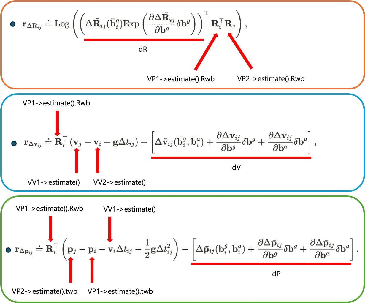
Here, the variables dR, dV, and dP are predictions of the system state in the residual function, calculated by integrating the state change between two consecutive time points based on IMU sensor data. These values are implemented as separate functions to get their values, and the code below shows where the values are assigned to the dR, dV, and dP variables.
const Eigen::Matrix3d dR = mpInt->GetDeltaRotation(b1).cast<double>();
const Eigen::Vector3d dV = mpInt->GetDeltaVelocity(b1).cast<double>();
const Eigen::Vector3d dP = mpInt->GetDeltaPosition(b1).cast<double>();
C++
복사
The definitions of the functions GetDeltaRotation, GetDeltaVelocity, and GetDeltaPosition are shown in the code below, and you can see that they are implemented identically to the parts of the formula labeled dR, dV, and dP in Equation (45). Here, JRg, JVg, JVa, JPg, and JPa are the Jacobian matrices for updating the bias that we discussed in the first post.
Eigen::Matrix3f Preintegrated::GetDeltaRotation(const Bias &b_)
{
std::unique_lock<std::mutex> lock(mMutex);
Eigen::Vector3f dbg;
dbg << b_.bwx-b.bwx,b_.bwy-b.bwy,b_.bwz-b.bwz;
return NormalizeRotation(dR * Sophus::SO3f::exp(JRg * dbg).matrix());
}
Eigen::Vector3f Preintegrated::GetDeltaVelocity(const Bias &b_)
{
std::unique_lock<std::mutex> lock(mMutex);
Eigen::Vector3f dbg, dba;
dbg << b_.bwx-b.bwx,b_.bwy-b.bwy,b_.bwz-b.bwz;
dba << b_.bax-b.bax,b_.bay-b.bay,b_.baz-b.baz;
return dV + JVg * dbg + JVa * dba;
}
Eigen::Vector3f Preintegrated::GetDeltaPosition(const Bias &b_)
{
std::unique_lock<std::mutex> lock(mMutex);
Eigen::Vector3f dbg, dba;
dbg << b_.bwx-b.bwx,b_.bwy-b.bwy,b_.bwz-b.bwz;
dba << b_.bax-b.bax,b_.bay-b.bay,b_.baz-b.baz;
return dP + JPg * dbg + JPa * dba;
}
C++
복사
This implemented Residual function is used as a key element of the IMU Factor node, which describes the state change (rotation, velocity, position) between two keyframes when performing IMU Preintegration. The Residual function defines the error between the predicted and actual state values, which is used to construct the optimization expression. By minimizing the difference between the predicted and actual state variables calculated by integrating the IMU data, the optimization process is used to incrementally improve the precision of the system state estimation.
Defining the Jacobian matrix
Next, let's take a look at the Jacobian matrix, which is the vector derivative of a multivariate vector function, which in nonlinear optimization terms means the result of differentiating the residual function, which is a multivariate vector function, with the state variables. It represents how the residual function, which we need to minimize, changes as the state variable changes. Therefore, the Jacobian matrix can be understood as a matrix that contains important information about the direction and magnitude of the change in the residual function.
The implementation of the Jacobian matrix for IMU preintegration is implemented in the linearizeOplus function of the EdgeInertial class. In the code, the order of the partial derivatives is listed in terms of state variables, and in the paper it is listed in terms of residual functions, so it is difficult to understand at a glance. Therefore, to make the code easier to understand, I added a comment to the existing ORB-SLAM3 code // Comment (Dongwon Shin): Added a commentary with keywords.
void EdgeInertial::linearizeOplus()
{
const VertexPose* VP1 = static_cast<const VertexPose*>(_vertices[0]);
const VertexVelocity* VV1= static_cast<const VertexVelocity*>(_vertices[1]);
const VertexGyroBias* VG1= static_cast<const VertexGyroBias*>(_vertices[2]);
const VertexAccBias* VA1= static_cast<const VertexAccBias*>(_vertices[3]);
const VertexPose* VP2 = static_cast<const VertexPose*>(_vertices[4]);
const VertexVelocity* VV2= static_cast<const VertexVelocity*>(_vertices[5]);
const IMU::Bias b1(VA1->estimate()[0],VA1->estimate()[1],VA1->estimate()[2],VG1->estimate()[0],VG1->estimate()[1],VG1->estimate()[2]);
const IMU::Bias db = mpInt->GetDeltaBias(b1);
Eigen::Vector3d dbg;
dbg << db.bwx, db.bwy, db.bwz;
const Eigen::Matrix3d Rwb1 = VP1->estimate().Rwb;
const Eigen::Matrix3d Rbw1 = Rwb1.transpose();
const Eigen::Matrix3d Rwb2 = VP2->estimate().Rwb;
const Eigen::Matrix3d dR = mpInt->GetDeltaRotation(b1).cast<double>();
const Eigen::Matrix3d eR = dR.transpose()*Rbw1*Rwb2;
const Eigen::Vector3d er = LogSO3(eR);
const Eigen::Matrix3d invJr = InverseRightJacobianSO3(er);
// Jacobians wrt Pose 1
_jacobianOplus[0].setZero();
// Comment (Dongwon Shin): derivative of rotation residual w.r.t rotation i
_jacobianOplus[0].block<3,3>(0,0) = -invJr*Rwb2.transpose()*Rwb1; // OK
// Comment (Dongwon Shin): derivative of velocity residual w.r.t rotation i
_jacobianOplus[0].block<3,3>(3,0) = Sophus::SO3d::hat(Rbw1*(VV2->estimate() - VV1->estimate() - g*dt)); // OK
// Comment (Dongwon Shin): derivative of translation residual w.r.t rotation i
_jacobianOplus[0].block<3,3>(6,0) = Sophus::SO3d::hat(Rbw1*(VP2->estimate().twb - VP1->estimate().twb
- VV1->estimate()*dt - 0.5*g*dt*dt)); // OK
// translation
// Comment (Dongwon Shin): derivative of translation residual w.r.t position i
_jacobianOplus[0].block<3,3>(6,3) = -Eigen::Matrix3d::Identity(); // OK
// Jacobians wrt Velocity 1
_jacobianOplus[1].setZero();
// Comment (Dongwon Shin): derivative of velocity residual w.r.t velocity i
_jacobianOplus[1].block<3,3>(3,0) = -Rbw1; // OK
// Comment (Dongwon Shin): derivative of translation residual w.r.t velocity i
_jacobianOplus[1].block<3,3>(6,0) = -Rbw1*dt; // OK
// Jacobians wrt Gyro 1
_jacobianOplus[2].setZero();
// Comment (Dongwon Shin): derivative of rotation residual w.r.t gyro bias i
_jacobianOplus[2].block<3,3>(0,0) = -invJr*eR.transpose()*RightJacobianSO3(JRg*dbg)*JRg; // OK
// Comment (Dongwon Shin): derivative of velocity residual w.r.t gyro bias i
_jacobianOplus[2].block<3,3>(3,0) = -JVg; // OK
// Comment (Dongwon Shin): derivative of translation residual w.r.t gyro bias i
_jacobianOplus[2].block<3,3>(6,0) = -JPg; // OK
// Jacobians wrt Accelerometer 1
_jacobianOplus[3].setZero();
// Comment (Dongwon Shin): derivative of velocity residual w.r.t acc bias i
_jacobianOplus[3].block<3,3>(3,0) = -JVa; // OK
// Comment (Dongwon Shin): derivative of translation residual w.r.t acc bias i
_jacobianOplus[3].block<3,3>(6,0) = -JPa; // OK
// Jacobians wrt Pose 2
_jacobianOplus[4].setZero();
// rotation
// Comment (Dongwon Shin): derivative of rotation residual w.r.t rotation j
_jacobianOplus[4].block<3,3>(0,0) = invJr; // OK
// translation
// Comment (Dongwon Shin): derivative of translation residual w.r.t position j
_jacobianOplus[4].block<3,3>(6,3) = Rbw1*Rwb2; // OK
// Jacobians wrt Velocity 2
_jacobianOplus[5].setZero();
// Comment (Dongwon Shin): derivative of velocity residual w.r.t velocity j
_jacobianOplus[5].block<3,3>(3,0) = Rbw1; // OK
}
C++
복사
In the IMU preintegration paper, the derivation of the formula for the Jacobian matrix is described in the C. Jacobians of Residual Errors section of the Appendix as follows.
•
1) Jacobians of position residual
•
2) Jacobians of velocity residual
•
3) Jacobians of rotation residual
This summarizes the results of differentiating the residual functions for rotation, velocity, and translation with respect to the state variables below.
•
Rotation state variable for keyframe i
•
Rotation state variable for keyframe j
•
Pan state variable for keyframe i
•
Rotation state variable for keyframe j
•
Vector state variable for keyframe i
•
Vector state variable for keyframe j
•
Acceleration bias state variable for keyframe i
•
Angular Velocity Bias State Variable for Keyframe i
For example, in the Jacobian matrix code shown below, the derivative of rotation residual w.r.t rotation i is therotation residual function at i as a function of the rotation state variable , which in the paper means .
// Comment (Dongwon Shin): derivative of rotation residual w.r.t rotation i
_jacobianOplus[0].block<3,3>(0,0) = -invJr*Rwb2.transpose()*Rwb1; // OK
C++
복사
Comparing between the paper and the code in this way, we can see that the formula for the Jacobian matrix in the paper is implemented verbatim.
Wrapping up
At first, I was curious about how IMU preintegration is actually implemented in ORB-SLAM3, so I searched for data, and I even wrote a post explaining it myself. It's been a long time since I posted a blog post on the homepage, but in the future, I will summarize what I often study. While studying, I found that VINS-MONO, another representative visual inertial odometry method, performs IMU preintegration in a different way from ORB-SLAM3, so I will write a post about it next time. I will also try to write about Semantic SLAM and Deep learning based visual localization if I get a chance.
I'm usually only interested in IMU sensor fusion, but I feel like I've become a little more familiar with IMU preintegration this time by studying it. Recently, Apple is also hiring VIO/SLAM engineers to make metaverse devices such as VisionPro, and I feel that it is being used more and more in addition to autonomous driving and robotics.

Thank you for reading to the end :-)