
Introduction
Recently, while studying IMU preintegration, I suddenly wondered how IMU preintegration is implemented in ORB-SLAM3, so I analyzed it. The theoretical part of IMU preintegration is already well explained Dr. Lim's blog, so I think it would be good to refer to it, and I compared the IMU preintegration paper with the ORB-SLAM3 code to see how the formula in the paper is implemented in the code.
It would take a lot of time to write the IMU preintegration part in one article, so I would like to write it in the following order.
1.
IMU sensor measurement integration
2.
Defining the residual function
3.
Definition of Jacobian matrix
This article will cover the code analysis of the first of them, IMU sensor measurement integration.
Code analysis
Integrating IMU Sensor Measurements
First, let's look at the part of the code that integrates the measurements between keyframe i and keyframe j by accumulating the acceleration and angular velocity measurements from the IMU sensor as they come in. During this process, the following values are computed
1.
The relative state (rotation, translation, velocity) values between the two keyframes.
2.
The covariance matrix used for noise propagation to perform optimization later on
3.
A Jacobian matrix for updating the bias.
The overall calculation is performed in the IntegrateNewMeasurement function of the Preintegrated class. The complete function code is shown below.
void Preintegrated::IntegrateNewMeasurement(const Eigen::Vector3f &acceleration, const Eigen::Vector3f &angVel, const float &dt)
{
mvMeasurements.push_back(integrable(acceleration,angVel,dt));
// Position is updated firstly, as it depends on previously computed velocity and rotation.
// Velocity is updated secondly, as it depends on previously computed rotation.
// Rotation is the last to be updated.
//Matrices to compute covariance
Eigen::Matrix<float,9,9> A;
A.setIdentity();
Eigen::Matrix<float,9,6> B;
B.setZero();
Eigen::Vector3f acc, accW;
acc << acceleration(0)-b.bax, acceleration(1)-b.bay, acceleration(2)-b.baz;
accW << angVel(0)-b.bwx, angVel(1)-b.bwy, angVel(2)-b.bwz;
avgA = (dT*avgA + dR*acc*dt)/(dT+dt);
avgW = (dT*avgW + accW*dt)/(dT+dt);
// Update delta position dP and velocity dV (rely on no-updated delta rotation)
dP = dP + dV*dt + 0.5f*dR*acc*dt*dt;
dV = dV + dR*acc*dt;
// Compute velocity and position parts of matrices A and B (rely on non-updated delta rotation)
Eigen::Matrix<float,3,3> Wacc = Sophus::SO3f::hat(acc);
A.block<3,3>(3,0) = -dR*dt*Wacc;
A.block<3,3>(6,0) = -0.5f*dR*dt*dt*Wacc;
A.block<3,3>(6,3) = Eigen::DiagonalMatrix<float,3>(dt, dt, dt);
B.block<3,3>(3,3) = dR*dt;
B.block<3,3>(6,3) = 0.5f*dR*dt*dt;
// Update position and velocity jacobians wrt bias correction
JPa = JPa + JVa*dt -0.5f*dR*dt*dt;
JPg = JPg + JVg*dt -0.5f*dR*dt*dt*Wacc*JRg;
JVa = JVa - dR*dt;
JVg = JVg - dR*dt*Wacc*JRg;
// Update delta rotation
IntegratedRotation dRi(angVel,b,dt);
dR = NormalizeRotation(dR*dRi.deltaR);
// Compute rotation parts of matrices A and B
A.block<3,3>(0,0) = dRi.deltaR.transpose();
B.block<3,3>(0,0) = dRi.rightJ*dt;
// Update covariance
C.block<9,9>(0,0) = A * C.block<9,9>(0,0) * A.transpose() + B*Nga*B.transpose();
C.block<6,6>(9,9) += NgaWalk;
// Update rotation jacobian wrt bias correction
JRg = dRi.deltaR.transpose()*JRg - dRi.rightJ*dt;
// Total integrated time
dT += dt;
}
C++
복사
It's hard to understand at a glance because it's a jumbled mess of calculations, so let's take a look at the three parts mentioned above in order.
Relative motion increments
In the Imu preintegration paper, formula (33) defines the formula for relative motion increments.
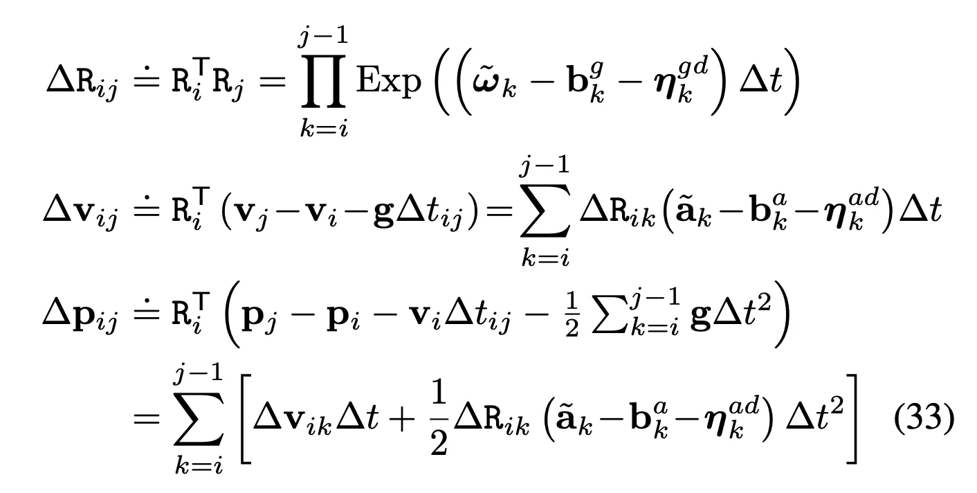
First, the term for position during relative motion increments in the code.
dP = dP + dV*dt + 0.5f*dR*acc*dt*dt;
C++
복사
Where acc represents the acceleration value in the form with the bias removed. The noise is modeled separately and used to create the covariance matrix, so we don't need to consider it here. And you'll notice that the symbol, which represents the sum, is expressed in the code as dP = dP + something.
Next, we need to add the terms for velocity, in the code looks like this, where acc can also be thought of as the expression mentioned above.
dV = dV + dR*acc*dt;
C++
복사
Next, we need to find the term for rotation, in the code.
IntegratedRotation dRi(angVel,b,dt);
dR = NormalizeRotation(dR*dRi.deltaR);
C++
복사
This part looks a little different from the code in the paper, but if you look at the constructor part of the IntegratedRotation class, you can see that the formula is written in the paper.
IntegratedRotation::IntegratedRotation(const Eigen::Vector3f &angVel, const Bias &imuBias, const float &time) {
const float x = (angVel(0)-imuBias.bwx)*time;
const float y = (angVel(1)-imuBias.bwy)*time;
const float z = (angVel(2)-imuBias.bwz)*time;
const float d2 = x*x+y*y+z*z;
const float d = sqrt(d2);
Eigen::Vector3f v;
v << x, y, z;
Eigen::Matrix3f W = Sophus::SO3f::hat(v);
if(d<eps)
{
deltaR = Eigen::Matrix3f::Identity() + W;
rightJ = Eigen::Matrix3f::Identity();
}
else
{
deltaR = Eigen::Matrix3f::Identity() + W*sin(d)/d + W*W*(1.0f-cos(d))/d2;
rightJ = Eigen::Matrix3f::Identity() - W*(1.0f-cos(d))/d2 + W*W*(d-sin(d))/(d2*d);
}
}
C++
복사
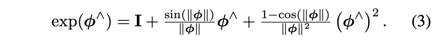
Here, the ) part of the formula is the code below, and the
const float x = (angVel(0)-imuBias.bwx)*time;
const float y = (angVel(1)-imuBias.bwy)*time;
const float z = (angVel(2)-imuBias.bwz)*time;
C++
복사
The code below is where the function is written to represent the exponential map.
Eigen::Matrix3f W = Sophus::SO3f::hat(v);
if(d<eps)
{
deltaR = Eigen::Matrix3f::Identity() + W;
rightJ = Eigen::Matrix3f::Identity();
}
else
{
deltaR = Eigen::Matrix3f::Identity() + W*sin(d)/d + W*W*(1.0f-cos(d))/d2;
rightJ = Eigen::Matrix3f::Identity() - W*(1.0f-cos(d))/d2 + W*W*(d-sin(d))/(d2*d);
}
C++
복사
Exponential maps are well described in the paper in equation (3).
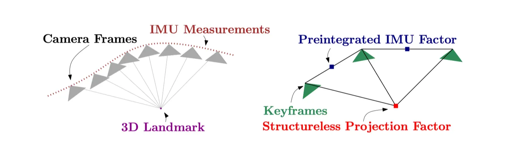
Using these terms, we can accumulate the continuously incoming IMU sensor acceleration and angular velocity values and estimate the relative motion between keyframes i and j. This relative motion is later used to perform bundle adjustment using keyframes, or to perform pose estimation for a single camera frame.
Covariance from noise propagation
Next, we need matrices A and B for noise propagation, which we talk about in the paper in equation (62).
However, the paper doesn't explicitly say how the matrices A and B are constructed; instead, the paper says that they are
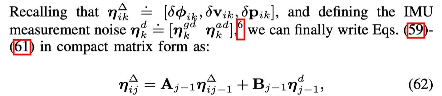
Therefore, by the definitions of it follows from equations (59)-(61) that and ], and the coefficient terms multiplied by ].
If we look in the code for the parts of the formula that correspond to matrices A and B, we can see that
// Compute velocity and position parts of matrices A and B (rely on non-updated delta rotation)
Eigen::Matrix<float,3,3> Wacc = Sophus::SO3f::hat(acc);
A.block<3,3>(3,0) = -dR*dt*Wacc;
A.block<3,3>(6,0) = -0.5f*dR*dt*dt*Wacc;
A.block<3,3>(6,3) = Eigen::DiagonalMatrix<float,3>(dt, dt, dt);
B.block<3,3>(3,3) = dR*dt;
B.block<3,3>(6,3) = 0.5f*dR*dt*dt;
(...)
// Compute rotation parts of matrices A and B
A.block<3,3>(0,0) = dRi.deltaR.transpose();
B.block<3,3>(0,0) = dRi.rightJ*dt;
C++
복사
If we compare the matrices A and B, we can see that the code is written the same as in the paper.
With matrices A and B organized, we can now find the covariance matrix.
// Update covariance
C.block<9,9>(0,0) = A * C.block<9,9>(0,0) * A.transpose() + B*Nga*B.transpose();
C.block<6,6>(9,9) += NgaWalk;
C++
복사
Note that the for the covariance matrix is represented by C in the code.
Jacobians used for the a bias update
Next, we need to calculate the Jacobians for the bias update. This part is unnumbered in the paper and is located above equation (70) in the Appendix. This is the result of differentiating the residual function by the acceleration and angular velocity bias terms.
// Update position and velocity jacobians wrt bias correction
JPa = JPa + JVa*dt -0.5f*dR*dt*dt;
JPg = JPg + JVg*dt -0.5f*dR*dt*dt*Wacc*JRg;
JVa = JVa - dR*dt;
JVg = JVg - dR*dt*Wacc*JRg;
(...)
// Update rotation jacobian wrt bias correction
JRg = dRi.deltaR.transpose()*JRg - dRi.rightJ*dt;
C++
복사
Where JPa is , JPg is , JVa is , JVg represents , and JRg represents . As you can see, the rotation values are only affected by the angular velocity bias, so we only perform a partial differentiation for the angular velocity bias. However, the velocity and position values are affected by both acceleration and angular velocity biases, so we perform a partial differentiation on both terms.
The Jacobian matrices here will be used to find the residual error, which will be discussed later.
Wrapping up
We have seen how the first part of the imu preintegration in the ORB-SLAM3 code, the IMU sensor measurement integration, is implemented. In the measurement integration part, we (1) compute the relative state (rotation, translation, velocity) values between two keyframes, (2) obtain the covariance matrix that is used to perform the optimization through noise propagation. We also (3) compute the Jacobian matrix for updating the bias and use these values later when performing bundle adjustment using keyframes, or when performing pose estimation for a single camera frame.
Next time, we will see how the Jacobian matrix is implemented in the paper to define and optimize the residual function between two keyframes using these defined relative motion increments.
Thanks for reading this long post :-)